
005 : Regression Modeling - Boston
This project utilizes linear regression on the Boston Housing dataset to predict house prices by optimizing a least squares loss function, aiming to model the relationship between various housing attributes and prices for accurate predictions.
Project Color Palette

The essence of data
This dataset contains information about houses in the Boston, Massachusetts area, United States.
The Boston Housing dataset consists of 506 samples and 13 attributes, detailing information about the surrounding environment of houses, such as the ratio of bathrooms, crime rates, distance to commercial centers and bus terminals, average apartment size nearby, and several other attributes:
- CRIM: Per capita crime rate by town.
- ZN: Proportion of residential land zoned for lots over 25,000 square feet.
- INDUS: Proportion of non-retail business acres per town.
- CHAS: Charles River dummy variable (1 if tract bounds river; 0 otherwise).
- NOX: Nitric oxides concentration.
- RM: Average number of rooms per dwelling.
- AGE: Proportion of owner-occupied units built prior to 1940.
- DIS: Weighted distances to five Boston employment centers.
- RAD: Index of accessibility to radial highways.
- TAX: Full-value property tax rate per $10,000.
- PTRATIO: Pupil-teacher ratio by town.
- B: 1000(Bk - 0.63)^2 where Bk is the proportion of Black people by town.
- LSTAT: Percentage of lower status population.
MEDV is the target variable for predicting house prices, serving as the attribute predicted by mathematical models.
To assess the essence of the data, evaluating the correlation and linear relationships among data points in scatter plots is crucial.
# Đọc dữ liệu từ file CSV vào DataFrame
df = pd.read_csv('https://raw.githubusercontent.com/selva86/datasets/master/BostonHousing.csv')
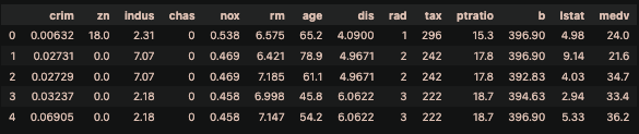
# Hiển thị 5 dòng đầu tiên của dữ liệu Boston
display(df.head())
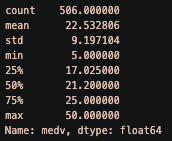
  # Thống kê mô tả của giá trị trung bình của giá nhà (MEDV)
  print(df['medv'].describe())
Approach and Methodology
A. Approach to the Problem:
The first step involves data preprocessing to explore correlations between attributes and the predictive target using a correlation matrix, as well as addressing outliers.
Following this approach, the dataset is split into training and testing sets.
Subsequently, linear regression is applied to predict house prices by optimizing a loss function based on the method of least squares.
By computing the inverse matrix of the transpose of the input matrix multiplied by the input matrix, optimal parameters for the linear regression model can be calculated.
Finally, the model is used to predict house prices on the test set, and the model's effectiveness is evaluated by computing the RMSE and R-squared metrics.
B. Least Squares Method:
The Least Squares Method has two variants: Univariable least square (used when only one independent variable predicts the dependent variable) and Multivariable least square (employed when multiple independent variables predict the dependent variable).
In this project, we'll be utilizing Multivariable least squares.
With Multivariable least squares, our goal is to find the best-fitting linear line to model the relationship between the dependent variable and multiple independent variables in multidimensional datasets.
The multivariable linear regression model is in the form of:
Y = β0 + β1X1 + β2X2 + … + βnXn + εIn which:
- Y is the dependent variable
- X1, X2, ..., Xn are the independent variables
- β0, β1, β2, ..., βn are the coefficients to be estimated
- ε is the residual error
θ̂ = (XTX)-1XTy = minθ ||y - Xθ||22In which:
- θ̂ is the column vector of optimal linear regression parameters.
- X is the design matrix with rows as samples and columns as features (including a column of all 1s for the intercept).
- y is the column vector of corresponding labels for each sample.
- Lack of linear relationship between independent and dependent variables.
- Presence of outliers.
- Correlation among residuals.
- Collinearity among independent variables.
In this project, we utilize the method of least squares to compute the parameters for the linear regression model.
This method is employed to determine a line that represents the linear relationship between the input and output variables.
The least squares method aims to find a line where the sum of squared errors on the training set is minimized.
Specifically, within our dataset, we use the input matrix X_train and the output vector y_train to compute the parameter vector θ using the method of least squares. The formula to calculate the parameter vector θ is as previously described.
Before computing the parameter vector θ, it's essential to check the invertibility of the matrix (XTX) by examining its determinant value. If the determinant equals zero, indicating the matrix is non-invertible, we cannot utilize the method of least squares to compute the parameter vector θ.
Model Initialization
A. Calculate the correlation matrix among the attributes:
The concept of the correlation matrix:
- The correlation matrix is a concept in statistics and linear algebra, commonly used to measure the linear relationship between attributes in a dataset.
- It's constructed by computing the correlation coefficients between each pair of attributes and organizing them into a square matrix.
- The values within the correlation matrix indicate the degree of correlation between attribute pairs.
- A value close to 1 signifies a strong linear relationship between two attributes; a value close to 0 implies no linear relationship between the attributes.
sns.heatmap(corr_matrix, annot=True, fmt=".1f", cmap ="crest")
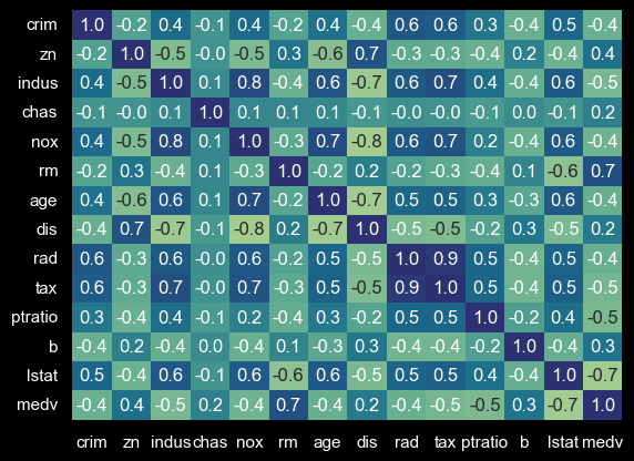
The heatmap reveals that the correlation coefficients of attributes RM (0.7 - positive correlation) and LSTAT (-0.7 - negative correlation) are the highest concerning the MEDV value we are computing.
To gain a clearer understanding of the distribution of these two attributes with the MEDV house prices, we'll employ a pairplot.
Concept of Pairplot:
- Pairplot is a visualization concept used to represent all pairwise relationships between attributes within a dataset.
- It's commonly depicted as a matrix of scatterplots, where each scatterplot signifies the linear relationship between two attributes.
ssns.pairplot(df[['rm', 'lstat', 'medv']])
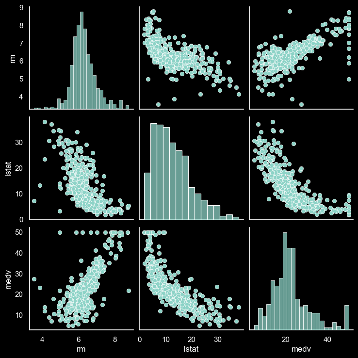
In the pairplot of the Boston housing dataset, we observe a linear relationship between house prices (MEDV) and the number of rooms (independent variable RM), as well as an inverse relationship with the lower status population ratio (independent variable LSTAT).
Specifically, when RM increases, MEDV (house prices) also tends to increase, while an increase in LSTAT leads to a decrease in MEDV.
Furthermore, the plot indicates a strong correlation (-0.6) between the two independent variables RM and LSTAT.
This might indicate multicollinearity between them.
Concept of Multicollinearity in Linear Regression:
- In linear regression, multicollinearity occurs when two or more independent variables in the model exhibit a strong correlation with each other.
- This could lead to inaccurate estimation of regression coefficients, reducing the model's accuracy and affecting its predictive capabilities.
- Multicollinearity is a crucial issue in data analysis and scientific research, requiring specific methods to identify and mitigate its impact.
- Techniques like using the Variance Inflation Factor (VIF) or performing a generalized eigenvalue decomposition can help identify the extent of multicollinearity and provide solutions to mitigate its effect on linear regression models.
Concept of Variance Inflation Factor (VIF):
- The Variance Inflation Factor (VIF) is used to assess the level of multicollinearity among independent variables in a linear regression model.
VIF indicates the magnitude of the variance of each independent variable after removing the effects of other independent variables on that variable. Therefore, if the VIF value for a particular independent variable is high, it suggests a greater likelihood of multicollinearity. -
VIF is calculated by determining the ratio of the variance of a multiple regression model with that variable to the variance of a simple linear regression model of that variable.
If the VIF value is greater than 1, the variable is considered to have multicollinearity effects.
Typically, if the VIF value exceeds 5 or 10, the variable is considered to be significantly multicollinear and needs to be addressed to mitigate the impact of multicollinearity on the regression model.
  # Chọn các biến độc lập và biến phụ thuộc
  Independent_vars = df[['rm', 'lstat']].values
  # Thêm một cột chứa giá trị 1 vào ma trận X để tính toán hệ số chặn
  Independent_vars = np.insert(Independent_vars, 0, 1, axis=1)
  # Tính toán VIF cho các biến độc lập
  vif = pd.DataFrame()
  vif["VIF Factor"] = [variance_inflation_factor(Independent_vars, i) for i in range(1, Independent_vars.shape[1])]
  vif["features"] = ['rm', 'lstat']
  # In kết quả
  print(vif)
| VIF Factor | Features |
|---|---|
| 1.60452 | rm |
| 1.60452 | lstat |
Based on the VIF results, we observe that both independent variables, RM and LSTAT, have VIF values less than 5.
Consequently, we can conclude that there is no multicollinearity between them.
Therefore, it is safe to use both independent variables in the linear regression model.
B. Handle the outliers:
Outliers can significantly influence the parameters of a linear model, especially the slope coefficient, as they can alter the slope of the linear line.
Their presence in the data can restrict the linear model from performing optimally as they can cause significant changes in the model's parameters.
This, in turn, may lead to inaccurate predictions and erroneous decisions.
Therefore, identifying and addressing outliers is crucial to achieve the best results from a linear model.
To identify outliers in the RM and LSTAT attributes, we employ the Interquartile Range (IQR) method to detect and subsequently remove them.
From the earlier pairplot, it's evident that RM follows a relatively normal distribution, while LSTAT exhibits a slightly left-skewed distribution.
  #Tính độ lệch của phân phối RM và LSTAT
  skew_rm = skew(df['rm'])
  skew_lstat = skew(df['lstat'])
  print(f"Độ lệch của rm: {skew_rm:.2f}")
  print(f"Độ lệch của lstat: {skew_lstat:.2f}")
| Features | Skewness |
|---|---|
| rm | 0.40 |
| lstat | 0.90 |
According to the computed results, the skewness of RM is 0.40, indicating that its distribution is closer to a normal distribution.
On the other hand, the skewness of LSTAT is 0.90, signifying a left-skewed distribution with many values concentrated in the left tail.
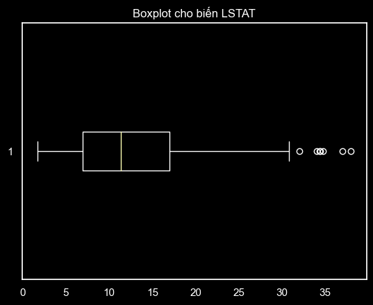
This observation aligns with the boxplot, where LSTAT exhibits numerous outliers on the right-hand side, highlighting its skewed distribution towards the lower values.
  # Vẽ boxplot cho biến lstat
  plt.boxplot(df['lstat'], vert= False)
  plt.title('Boxplot cho biến LSTAT')
  plt.show()
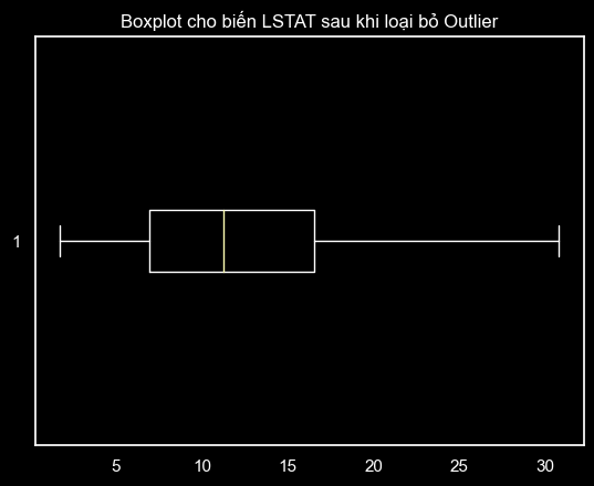
For RM, there might not be a necessity to handle outliers as the skewness is relatively low and its distribution is close to normal.
However, for LSTAT, it might be appropriate to employ outlier removal using the lower_bound and upper_bound values derived from the Interquartile Range (IQR) method, as mentioned earlier.
  #Tính IQR
  q1 = np.percentile(df['lstat'], 25)
  q3 = np.percentile(df['lstat'], 75)
  iqr = q3 - q1
  #Tính giá trị lower_bound và upper_bound
  lower_bound = q1 - 1.5 * iqr
  upper_bound = q3 + 1.5 * iqr

  #Loại bỏ các giá trị ngoại lai của LSTAT
  df = df[(df['lstat'] > lower_bound) & (df['lstat'] < upper_bound)]

  # Vẽ boxplot cho biến LSTAT sau khi loại bỏ Outlier
  plt.boxplot(df['lstat'], vert= False)
  plt.title('Boxplot cho biến LSTAT sau khi loại bỏ Outlier')
  plt.show()
C. Split the data to train and test:
  # Chọn các thuộc tính RM và LSTAT làm biến độc lập, MEDV làm biến phụ thuộc
  X = df[['rm', 'lstat']].values
  y = df['medv'].values

  # Thêm một cột chứa giá trị 1 vào ma trận X để tính toán hệ số chặn
  X = np.insert(X, 0, 1, axis=1)
  Chia dữ liệu thành tập train và tập test tỉ lệ 70:30
  X_train, X_test, y_train, y_test = train_test_split(X, y, test_size=0.3, random_state=42)
It inserts a column with a value of 1 into the X matrix to calculate the intercept coefficient.
Finally, it divides the data into training and testing sets with a 70:30 ratio.
D. Apply linear regression to predict house prices by optimizing the loss function using the method of least squares:
  #Kiểm tra ma trận X^T X có thể đảo ngược hay không
  XTX = X_train.T.dot(X_train)
  det = np.linalg.det(XTX)
  if det == 0:
      print("Ma trận X^T X không thể đảo ngược.")
  else:
      print("Ma trận X^T X có thể đảo ngược.")
  # Tính toán bộ tham số theta bằng phương pháp bình phương tối tiểu
  XT = np.transpose(X_train)
  XTX1 = np.linalg.inv(XT.dot(X_train))
  XTY = XT.dot(y_train)
  theta = XTX1.dot(XTY)
  print(theta)
  print(f"MEDV = {theta[0]} + {theta[1]} * RM + {theta[2]}* LSTAT")
The formula generated by the linear regression model is:
MEDV = 2.95 + 4.64 * RM - 0.75 * LSTATThe slope coefficient for RM is 4.64, indicating a positive correlation between RM and MEDV.
his means that as the value of RM increases, the value of MEDV also increases.
The slope coefficient for LSTAT is -0.75, indicating a negative correlation between LSTAT and MEDV.
This means that as the value of LSTAT increases, the value of MEDV decreases.
The intercept coefficient of the model is 2.95, indicating the value of MEDV when RM = 0 and LSTAT = 0 is 2.95.
These coefficients can be used to predict the value of MEDV based on RM and LSTAT for new datasets.
However, it's important to note that the model can only predict the accuracy of MEDV to the extent explained by RM and LSTAT, and there might be other factors influencing MEDV that this model does not include.
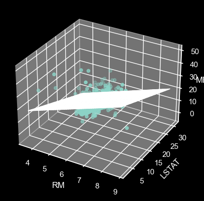
After obtaining the parameter set theta for the multivariate linear regression equation, we will represent it in the form of a plane in three-dimensional space corresponding to 2 independent variables (RM, LSTAT) and 1 dependent variable (MEDV):
  x_min = np.min(X[:, 1])
  x_max = np.max(X[:, 1])
  y_min = np.min(X[:, 2])
  y_max = np.max(X[:, 2])
  xx, yy = np.meshgrid(np.linspace(x_min, x_max), np.linspace(y_min, y_max))
  Z = theta[0] + theta[1] * xx + theta[2] * yy
  fig = plt.figure()
  ax = fig.add_subplot(111, projection='3d')
  ax.scatter(X[:, 1], X[:, 2], y)
  ax.plot_surface(xx, yy, Z, alpha=0.5)
  ax.set_xlabel('RM')
  ax.set_ylabel('LSTAT')
  ax.set_zlabel('MEDV')
  plt.show()
Experimental Evaluation
  # Dự đoán giá trị nhà cho tập kiểm tra
  y_pred = np.dot(X_test, theta)
  residuals = y_test - y_pred
  fig, (ax1, ax2) = plt.subplots(1, 2, figsize=(10, 4))

  # Vẽ biểu đồ so sánh giá trị thực tế và giá trị dự đoán
  ax1.scatter(y_test, y_pred, alpha=0.5)
  ax1.plot([0, max(y_test)], [0, max(y_test)], '--', color='red')
  ax1.set_xlabel('Giá trị thực tế')
  ax1.set_ylabel('Giá trị dự đoán')
  ax1.set_title('Biểu đồ so sánh giá trị thực tế và giá trị dự đoán')

  # Vẽ đồ thị Residual Plot
  ax2.scatter(y_pred, residuals)
  ax2.axhline(y=0, color='r', linestyle='-')
  ax2.set_xlabel('Giá trị dự đoán')
  ax2.set_ylabel('Sai số (Residual)')
  ax2.set_title('Biểu đồ phân tán của sai số')

  plt.tight_layout()
  plt.show()
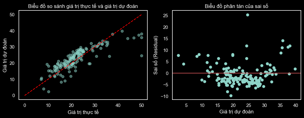
- In the first plot (on the left), we compare the actual values with the predicted values. The points are represented by blue dots. The red line represents the diagonal line (y = x), indicating the similarity between the actual and predicted values. If the data points lie close to the diagonal line (the red line), the model predicts well. Conversely, if the data points are far from the diagonal line, the model's predictions are not accurate.
- In this first plot, considering the overall values, it can be observed that the model tends to predict lower than the actual values when the actual values are greater than around 30. However, for lower actual values, the model predictions are relatively accurate.
- In the second plot (on the right), we represent the residuals using blue dots. The red line is the y = 0 line, representing the case where there are no residuals. If the points are evenly distributed around this line, we can conclude that the linear regression model is good.
- The residual plot in the housing price prediction example shows that the residuals are randomly distributed around the mean value of 0. This indicates that the linear regression model has met the requirements of randomness and independence among the data points. This ensures the reliability of predictions and the applicability of the model to new cases.
- However, there are still some data points far from the mean line, suggesting that the model hasn't fully captured the variations in the data. This could be due to the model's dependence on assumptions about distribution and correlation among the input variables or the presence of outliers or abnormal data. These data points need further investigation to determine the cause and improve the model if necessary.
B. Evaluate the effectiveness of the obtained equation based on RMSE and R-squared
The concept of RMSE:
RMSE is calculated using the mathematical formula as follows:
RMSE = √( 1⁄ n Σ i=1 n ( ytest_i - ypred_i )2 )In which:
- RMSE is Root Mean Square Error
- n is the number of data points
- y_test_i is the actual value of the i-th data point
- y_pred_i is the predicted value of the i-th data point
  # Tính toán sai số RMSE
  rmse = np.sqrt(np.mean((y_test - y_pred) ** 2))
  # Tính giá trị trung bình của biến mục tiêu
  y_mean = np.mean(y_test)
  print('Giá trị trung bình của biến mục tiêu:', y_mean)
  print('RMSE:', rmse)

  # Nhận xét kết quả
  if rmse < y_mean:
      print('RMSE nhỏ hơn giá trị trung bình của biến mục tiêu, mô hình có độ chính xác tương đối tốt.')
  else:
      print('RMSE lớn hơn giá trị trung bình của biến mục tiêu, mô hình có độ chính xác tương đối thấp.')
RMSE: 4.73.
As the RMSE is smaller than the average value of the target variable, the model shows relatively good accuracy.
Concept of R-squared:
- R-squared (R2) is a statistical metric used to assess the accuracy of a regression model.
- R2 indicates the percentage of variance in the target variable (explained by the model) that is explained by the independent variables in the model.
- R2 ranges from 0 to 1, and the closer its value is to 1, the better the model fits the data.
R2 = 1 - SSres⁄SStotIn which:
SSres = ∑i=1(ytest_i - ypred_i)2
SStot = ∑i=1(ytest_i - ȳ)2
- ytest_i is the actual value of the i-th data sample
- ypred_i is the predicted value of the i-th data sample
- ȳ is the mean value of the target variable (in this case, house prices), and n is the number of data samples.
Both SSres and SStot are calculated by summing the squared differences between the predicted value and the actual value.
R2 has significant importance in evaluating regression models. A higher R2 value indicates that the model explains a large portion of the variability of the target variable and hence is a better model.
  #Tính R-squared
  SS_res = sum((y_test - y_pred)**2)
  SS_tot = sum((y_test - y_mean)**2)
  R_squared = (1 - SS_res/SS_tot)

  print(R_squared)
The R-square value of 0.68 indicates that the model explains approximately 68% of the variability of the dependent variable using the independent variables in the model.
C. Further development direction
The result of the housing price prediction model in Boston based on two independent variables, RM and LSTAT, shows that the model has a relatively good predictive capability.
The R-square result of the model is 0.68, indicating that 68% of the variance in house prices is explained by the two independent variables RM and LSTAT. Additionally, the residual plot displays a concentration of data points around the mean line. However, there are still some outliers and uneven error amplitudes, which may need further investigation to optimize the model.
Some suggestions to improve the model's performance include:
- Using additional independent variables like TAX, AGE, NOX, DIS to analyze their impact on house prices.
- Applying data preprocessing methods such as normalization, transformation, handling missing data to minimize the influence of noise and outliers on the results.
- Experimenting and comparing the effectiveness of other models like Random Forest, Decision Tree, SVM to find the most suitable model for the data and better explain the independent variables.